SKEW-T DIAGRAM


A legend explaining the isopleths on the Skew-T is here.
A sample sounding is here.
An Air Weather Service (USAF) publication on Skew-T analysis is here (AWSTR 79-006).


1. Moisture content (RH, w, ws, e, es) 11. Stratus dissipation (method)
2. Forecasting surface temps (Tmax, Tmin) 12. Contrails (method)
3. Theoretical temps (Tw, theta, thetaw, Tv) 13. Stability indices (definitions, lifted layer)
4. Thickness (method, snow index) 14. Stability indices (SI, LI)
5. Mechanical lift (LCLp, LFCp, ELp) 15. Stability indices (FMI, KI)
6. Convective lift (CCLp, Tp, ELp) 16. Stability indices (TTI, SW)
7. Convective lift (CCLML, TCML, ELCML) 17. TS elements (T1, T1A for gusts)
8. Turbulent lift (MCLML) 18. TS elements (T2 for gusts; hailsize)
9. Inversions (radiation, subsidence, frontal, turbulent)
10. Fog dissipation (method)


MOISTURE CONTENT


Relative Humidity (RH) =
  1. w/ws x 100 %
  2. e/es x 100 %
Mixing Ratio (w)
  1. At p, find Td.
  2. Read w scale.
  3. Label in g/kg.
Vapor Pressure (e)
  1. At p, find Td.
  2. Extend a line isothermally to 622 mb (hPa).
  3. Read w scale; label in mb (hPa).
Saturation Mixing Ratio (ws)
  1. At p, find T.
  2. Read w scale.
  3. Label in g/kg.
Saturation Vapor Pressure (es)
  1. At p, find T.
  2. Extend a line isothermally to 622 mb (hPa).
  3. Read w scale; label in mb (hPa).


FORECASTING SURFACE
TEMPERATURES


Maximum Temperature (TMAX)
  1. At 850 mb (hPa), find T.
  2. CLR - SCT: Extend line dry-adiabatically to surface.
  3. BKN - OVC: Extend line moist-adiabatically to surface.
  4. Read temperature scale.

If there is an inversion present with top between 4000 and 6000 ft AGL:
  1. Find T at warmest point in inversion.
  2. Extend a line dry-adiabatically to surface.
  3. Read temperature scale.
Minimum Temperature (TMIN)
  1. At 850 mb (hPa), find Td.
  2. Extend line moist-adiabatically to surface.
  3. Read temperature scale.


Alternate method:
  1. Find max temp; read Td.
  2. Td will be following morning's min T.
  3. Most accurate with CLR-SCT sky and light and variable wind.


THEORETICAL TEMPERATURES


Wet-Bulb Temperature (Tw)
  1. At p, find LCL.
  2. Extend a line moist-adiabatically to p.
  3. Read temperature scale.
Wet-Bulb Potential Temperature (thetaw)
  1. At p, find LCL or Tw.
  2. Extend a line moist-adiabatically to 1000 mb (hPa).
  3. Read temperature scale.
Potential Temperature (theta)
  1. At p, find T.
  2. Extend a line dry-adiabatically to 1000 mb (hPa).
  3. Read temperature scale.
Virtual Temperature (Tv)
  1. At p, find T and w. Read T in dC and w in g/kg.
  2. Use equation: Tv = T + w/6.


THICKNESS
(Delta-Z)


Method:
  1. Compute and plot Tv curve.
  2. Find mean Tv using equal area method (Tv and isotherm).
  3. Where mean Tv crosses thickness scale, read value.
  4. Label in feet or meters.
Snow Index:

y + 2x = N


y = 850 to 700 mb (hPa) delta-z
x = 1000 to 850 mb (hPa) delta-z


Scale:
  1. More than 4179 meters = Rain.
  2. Equal to 4179 meters = Mixed.
  3. Less than 4179 meters = Snow.


MECHANICAL LIFT
(PARCEL METHOD)


Diagrams illustrating this are
here and here.

Lifted Condensation Level (LCL)
  1. At p, find Td.
  2. Extend upward parallel to the mixing ratio line.
  3. At p, find T.
  4. Extend a line dry-adiabatically to intersect line from step 2.
  5. Read p, label in mb (hPa).
Level of Free Convection (LFC)
  1. From surface LCL, extend a line moist-adiabatically to T profile.
  2. Read LFC in mb (hPa).
Equilibrium Level (EL)
  1. From LFC (or LCL, if above the LFC), extend a line moist-adiabatically to T profile.
  2. Read EL in mb (hPa).


CONVECTIVE LIFT
(PARCEL METHOD)


A diagram illustrating this is
here.

Convective Condensation Level (CCL)
  1. At surface, find Td.
  2. Extend a line parallel to constant mixing ratio line and intersect T profile.
  3. Read pressure scale.
Convective Temperature (Tc)
  1. Find CCL.
  2. Extend a line dry-adiabatically to surface, read T.
Equilibrium Level (EL)
  1. From CCL, extend a line moist-adiabatically to T profile.
  2. Read EL in mb (hPa).


CONVECTIVE LIFT
(MOIST LAYER METHOD)


Convective Condensation Level (CCL)
  1. Determine top of moist layer: Dew-point depression greater than 6 degrees Celsius; if greater than 6000 feet, use lowest 150 mb (hPa) as moist layer.
  2. Find mean mixing ratio using equal area method: Td and w or isotherm.
  3. Extend a line parallel to constant mixing ratio line and intersect T profile.
Convective Temperature (Tc)
  1. Find CCL.
  2. Extend a line moist-adiabatically to surface, read T.
Equilibrium Level (EL)
  1. From CCL, extend a line moist-adiabatically to T profile.
  2. Read EL in mb (hPa).


TURBULENT LIFT


Mixing Condensation Level (MCL)
  1. Find top of mixed layer.
  2. Find mean mixing ratio using equal area method (mixing ratio line and Td).
  3. Extend a a line parallel to constant mixing ratio line to top of mixed layer.
  4. Find mean potential temperature using equal area method.
  5. Extend a line dry-adiabatically from the mean potential temperature to the top of the mixed layer.
  6. If line from step 3 and line from step 5 intersect within layer, read p in mb (hPa). If not, there is no MCL.


INVERSIONS


Radiation Inversion (illustration here)
  1. Surface based.
  2. Often T = Td or T ~ Td at surface.
  3. Tdwill be almost parallel to mixing ratio line within the inversion.
  4. T and Td cools above the inversion.
Frontal Inversion (illustration here)
  1. T is shallow isothermal or stable in inversion.
  2. Td increases within inversion.
Subsidence Inversion (illustration here)
  1. T increases in inversion.
  2. Td rapidly decreases in inversion.
  3. T cools approximately dry-adiabatically above inversion.
Turbulence Inversion
  1. T is dry-adiabatic below inversion.
  2. Td is parallel to mixing ratio lines below the inversion.
  3. T is isothermal in the inversion.


FORECASTING RADIATION
FOG DISSIPATION


Legend
  1. wa = Surface mixing ratio.
  2. wb = Inversion-top mixing ratio.
  3. w' = Mean mixing ratio =

    (wa + wb)/2

  4. Tx = Intersection temp (w and T).
  5. dT = Fog dissipation temp.
  6. DT = dT - Tx.
Method
  1. Determine wa and wb.
  2. Determine w' using formula; plot.
  3. Read Tx at lowest intersection of w and T.
  4. From Tx extend a line dry-adiabatically to surface: Read dT.
  5. Find DT; multiply by 328 feet for fog depth.

DO NOT USE HEIGHT SCALE


FORECASTING STRATUS
DISSIPATION


Legend
  1. wa = Surface mixing ratio.
  2. wb = Inversion-base mixing ratio.
  3. w' = Representative mixing ratio =

    (((wa + wb)/2)+Wa)/2

  4. Tx1 = First intersection w' and temp (base of stratus).
  5. Tx2 = Second intersection w' and temp (top of stratus).
  6. dT1 = Stratus dissipation beginning temperature.
  7. dT2 = Stratus dissipation ending temperature.
  8. DT1 = dT1 - Tx1.
  9. DT2 = dT2 - Tx2.
Method
  1. Determine wa and wb.
  2. Determine w' using formula; plot.
  3. Read Tx1 and Tx2.
  4. From Tx1 and Tx2, extend lines dry-adiabatically to surface.
  5. Read dT1 and dT2.
  6. Find DT1 and DT2.
  7. Stratus base = DT1 x 328 feet.
  8. Stratus top = DT2 x 328 feet.

DO NOT USE HEIGHT SCALE


FORECASTING CONDENSATION
TRAILS (CONTRAILS)


Method
  1. If forecasting clear-scattered conditions at cirrus levels, draw in 40 % RH line.
  2. If forecasting cloud deck in vicinity of tropopause, or broken-overcast clouds at cirrus levels, draw in 70 % RH line.
  3. Using temperature profile, forecast contrails to the left of the 40 % or 70 % RH line, depending on cloud forecast.
  4. Label contrail area boundaries in mb (hPa).


STABILITY INDICES


Definitions (illustration here)
  1. Absolutely stable: lapse rate .lt. moist adiabatic rate .lt. dry adiabatic rate.
  2. Absolutely unstable: moist adiabatic rate .lt. dry adiabatic rate .lt. lapse rate.
  3. Conditional states: moist adiabatic rate .lt. lapse rate .lt. dry adiabatic rate.
DPD = 0 -> Conditionally unstable
DPD > 0 -> Conditionally stable
Stability of a lifted layer
  1. Lift layer desired number of mb (hPa) by lifting both base and top the same distance.
  2. Lift temperature dry-adiabatically until saturation, then moist adiabatically remainder of distance.
  3. Construct new temperature curve by connecting base and top of lifted layer.
  4. Check stability indices.


Showalter Stability Index (SI)
  1. Find LCL for 850 mb (hPa).
  2. From LCL, extend a line moist-adiabatically to 500 mb (hPa).
  3. Read Tparcel at 500 mb (hPa).
  4. Read Tenvironment at 500 mb (hPa).
  5. Use formula: SSI = Tenvironment - Tparcel.
Lifted Index (LI) [Moist layer method]
  1. In lowest 100 mb (hPa), bisect Td with w to determine mean w (wm).
  2. In lowest 100 mb (hPa), determine mean T using an isotherm (Tm).
  3. Plot wm and Tm 50 mb (hPa) above the surface.
  4. Determine LCL using above.
  5. From intersection, extend a line moist-adiabatically to 500 mb (hPa).
  6. Read Tparcel at 500 mb (hPa).
  7. Read Tenvironment at 500 mb (hPa).
  8. Use formula: LI = Tenvironment - Tparcel.

Note: The LI can also be computed by simply using the surface T and Td.
SCALE

+1 .lt. SI .le. +3 RASH/SNSH probable; TS possible
-3 .lt. SI .le. +1 TS probable
-6 .lt. SI .le. -3 TS+ possible
SI .le. -6 Tornado possible
SCALE

0 .lt. LI .le. +2 RASH/SNSH probable; TS possible
-4 .lt. LI .le. 0 TS probable
-7 .lt. LI .le. -4 TS+ possible
LI .le. -7 Tornado possible


Fawbush-Miller Index (FMI)
  1. Determine moist layer.
  2. In moist layer, bisect Tw curve with w or isotherm to form equal areas.
  3. From bisection point, extend a line moist adiabatically to 500 mb (hPa); read T'.
  4. Use formula: FMI = T500 - T'.
K Index (KI)

KI = (T + Td)850 - (T - Td)700 - T500.

SCALE

.gt. 1 Relatively stable
0 to -2 Slightly unstable
- 2 to -6 Moderately unstable
.le. -7 Strongly unstable
SCALE (Airmass TS Probability)

.lt. 15 0 %
15 to 20 20 %
21 to 25 20 to 40 %
26 to 30 40 to 60 %
31 to 35 60 to 80 %
36 to 40 80 to 90 %
.gt. 40 ~ 100 %


Total-Totals Index (TT)

TT = (T + Td)850 - (2 x T500).

Severe Weather Threat Index (SW)

SW = 12D + 20(TT - 49) + 2f8 + f5 + VT

  1. D = 850 mb (hPa) Td. If .le. 0, D = 0.
  2. TT = Total totals index. If TT .le. 49, entire term is set to zero.
  3. f8 = 850 mb (hPa) wind speed (kts).
  4. f5 = 500 mb (hPa) wind speed (kts).
  5. VT = Veering Term = 125(S - 0.20), where S = sine of the angle between 850 mb (hPa) and 500 mb (hPa) winds.

Note: VT = 0 if any of the following apply:
Either 850 mb (hPa) or 500 mb (hPa) wind speed is less than 15 knots.
850 mb (hPa) wind NOT between 130 degrees to 250 degrees inclusive.
500 mb (hPa) wind not between 210 degrees and 310 degrees inclusive.
850 mb (hPa) to 500 mb (hPa) wind direction doesn't veer.
SCALE (Severe Weather Probability)
.ge. 49 Weak
50 to 55 Moderate
.ge. 56 Strong
SCALE
.gt. 400 Tornadoes
.ge. 300 to .lt. 400 TS+
.lt. 300 Disregard


FORECASTING THUNDERSTORM
ELEMENTS


T1 Method for TS Gusts (Inverson Present)
  1. From warmest point of inversion, extend a line moist-adiabatically to 600 mb (hPa).
  2. Label B' on isotherm scale. B = T600.
  3. See AWSTR 200, pg. 10-4 for uncorrected gust speed (v') (see below).
  4. Add 1/3 mean wind speed, surface to 5000 feet (v) to v' for max gust speed.
  5. Direction is wind direction between 10,000 and 14,000 feet, or use VRB.
T1 Method for TS Gusts (No Inverson)
  1. Forecast TMAX using clear-scattered method.
  2. Extend a line moist-adiabatically to 600 mb (hPa) and label B' on isotherm scale. B = T600.
  3. See AWSTR 200, pg. 10-4 for uncorrected gust speed (v') (see below).
  4. Add 1/3 mean wind speed, surface to 5000 feet (v) to v' for max gust speed.
  5. Direction is wind direction between 10,000 and 14,000 feet, or use VRB.


Table from AWSTR 200 Page 10-4
Use of T1 Method for Maximum Wind Gusts

T1 values in dC
Maximum gust speed (v') in knots
3
17
4
20
5
23
6
26
7
29
8
32
9
35
10
37
11
39
12
41
13
45
14
47
15
49
16
51
17
53
18
55
19
57
20
58
21
60
22
61
23
63
24
64
25
65


T2 Method for TS Gusts
  1. Find downrush temperature (TDR) by extending a line moist-adiabatically from wet-bulb zero (WBZ) to surface.
  2. Find TMAX using clear-scattered method.
  3. T2 = TMAX - TDR.
  4. See AWSTR 200, pg. 10-5 for max gust (see below). Note 3 values, but forecast the highest.
  5. Direction is wind direction between 10,000 and 14,000 feet, or use VRB.
Hailsize
  1. Draw two reference lines: pressure-level of CCLML and pressure-level of -5 dC on T profile.
  2. At intersection of T and CCLML, extend a line moist-adiabatically to second reference line. Label B'.
  3. Label -5 dC point as B. Base - B' - B.
  4. From 0 dC isotherm on second reference line, extend a line dry-adiabatically to first reference line. Label H' on isotherm scale.
  5. Label point on second reference line as H. Altitude = H' - H.
  6. See AWSTR 200, pg. 9-2 for uncorrected hail size (see below).
  7. If WBZ .ge. 10,000 ft AGL, see See AWSTR 200, pg. 9-4 for corrected hail size (see below).
  8. If WBZ .lt. 10,000 ft AGL, no correction is needed.


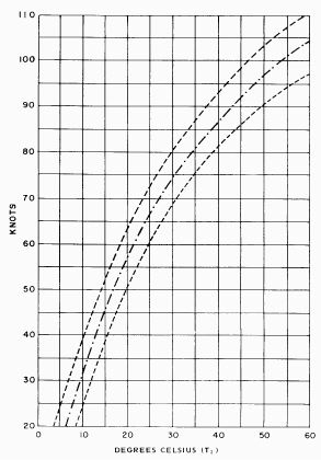
Figure from AWSTR 200 Page 10-5
Use of T2 Alternate Method for Maximum Wind Gusts


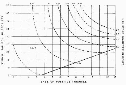
Figure from AWSTR 200 Page 9-2
Uncorrected Hail Size


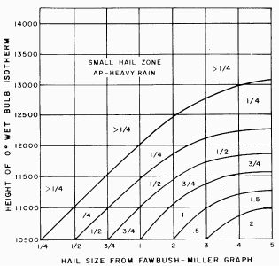
Figure from AWSTR 200 Page 9-4
Corrected Hail Size


SOURCES


_____, 1979: The Use of the Skew T, Log P Diagram in Analysis and Forecasting (AWS/TR-79/006 -- Revised), Air Weather Service (MAC), United States Air Force.

Miller, Robert C., 1975: Notes on Analysis and Severe-Storm Forecasting Procedures of the Air Force Global Weather Central (Technical Report 200 -- Revised), Air Weather Service (MAC), United States Air Force.

Miller, Sam, 2015: Applied Thermodynamics for Meteorologists, Cambridge University Press, 385 pgs.


This page was last updated on 02/26/2025.